

Modelling vaccination schedules for a cancer immunoprevention vaccine
- Research
- Open Access
Modelling vaccination schedules for a cancer immunoprevention vaccine
- Received: 09 June 2005
- Accepted: 07 October 2005
- Published: 07 October 2005
Abstract
We present a systematic approach to search for an effective vaccination schedule using mathematical computerized models. Our study is based on our previous model that simulates the cancer vs immune system competition activated by tumor vaccine. This model accurately reproduces in-vivo experiments results on HER-2/neu mice treated with the immuno-prevention cancer vaccine (Triplex) for mammary carcinoma. In vivo experiments have shown the effectiveness of Triplex vaccine in protection of mice from mammary carcinoma. The full protection was conferred using chronic (prophylactic) vaccination protocol while therapeutic vaccination was less effcient.
In the present paper we use the computer simulations to systematically search for a vaccination schedule which prevents solid tumor formation. The strategy we used for defining a successful vaccination schedule is to control the number of cancer cells with vaccination cycles. We found that, applying the vaccination scheme used in in-vivo experiments, the number of vaccine injections can be reduced roughly by 30%.
Keywords
- Antigen Present Cell
- Mammary Carcinoma
- Tumor Associate Antigen
- Vaccine Cell
- Molecular Entity
1 Introduction
Tumor immunologists have long sought ways to turn experimental results into effective therapies for human cancer patients. The best results so far are provided by using various monoclonal antibodies directed against tumor cells, which won approval from regulatory agencies and entered clinical practice. Other approaches, such as therapeutic vaccines that aim at stimulating the immune response of the host against tumor cells, were much less successful [1]. Experimental evidence clearly shows that vaccines elicit effective responses against early, microscopic tumors, but are ineffective against established, large tumor masses. A similar situation is found in infectious immunity: prophylactic vaccines protect millions of individuals worldwide from pathogens, whereas therapeutic vaccines are mostly ineffective. Such results led some tumor immunologists to the idea that the effort should be directed towards the development of prophylactic, rather than therapeutic, cancer vaccines [2]. Prophylactic vaccines against viruses that increase the risk of cancer, such as hepatitis B virus (HBV) or papilloma virus (HPV), have already shown a significant effcacy in reducing cancer incidence [3, 4]. The challenge is now to devise immunological strategies for the design of prophylactic vaccines for prevention of those human cancers that are not related to viral infections.
Standard vaccines against viruses induce the primary response of the adaptive components of the immune system against the non-self antigen in order to activate the immune system memory which will then elicit the much stronger secondary response when the antigen will enter the body. There is no need to break self tolerance as the antigen is non self.
At variance tumor vaccines need to break tolerance of the tumor associated antigens (TAA) that otherwise would be treated as self and not attacked by the immune system.
The effectiveness of tumor immuno-prevention was demonstrated in the past ten years in several mouse models of tumor development. Tumors in these models are induced either by chemical carcinogens or by transgenic expression of oncogenes. Among the most thoroughly investigated is the HER-2/neu transgenic mouse model. HER-2/neu is an oncogene involved in human breast and ovary carcinomas. The protein product of HER-2/neu, p185neu, is a membrane tyrosine kinase that transduces proliferative signals. A deregulation of HER-2/neu, for example due to gene amplification, leads to uncontrolled cell proliferation. Over-expression of a rat HER-2/neu transgene in mice was obtained using tissue-specific regulatory sequences derived from mammary tumor virus (MMTV) long terminal repeats (LTR). Various transgenic mouse lines were obtained using either a mutant, constitutively activated HER-2/neu gene or a normal, non mutated gene. Here we will refer to mice carrying the mutant oncogene, which are prone to a very aggressive mammary carcinogenesis, invariably leading to the development of invasive mammary carcinomas by the age of 6 months. The natural history of mammary carcinoma in HER-2/neu transgenic mice was thoroughly investigated and found to be remarkably similar to that of human breast cancer [5]. Immuno-prevention of mammary carcinoma in HER-2/neu transgenic mice was attempted using various immunological strategies, including cytokines, non-specific stimulators of the immune response, and HER-2/neu specific vaccines made of DNA, proteins, peptides, or whole cells. Most approaches achieved a delay of mammary carcinogenesis, but a complete prevention of tumor onset was not attained, particularly in the most aggressive tumor models [6]. We achieved the first complete success at preventing mammary carcinoma in HER-2/neu transgenic mice using a vaccine that combined three different stimuli for the immune system. The first was p185neu, protein product of HER-2/neu, which in this system is at same time the oncogene driving carcinogenesis and the target antigen. p185neu was combined with the two non specific adjuvants, allogeneic class I major histocompatibility complex (MHCI) glycoproteins and interleukin 12 (IL-12). MHCI glycoproteins are responsible for some of the most intense immune responses observed during the rejection of allogeneic organ transplants. Unlike conventional antigens, allogeneic MHCI molecules stimulate a relatively large fraction of all T cell clones, up to 10% of the available repertoire. IL-12 is a cytokine normally produced by antigen presenting cells (APC) such as dendritic cells (DC) to stimulate T helper cells and other cells of the immune system, such as natural killer cells (NK) [7]. IL-12 was initially administered systemically, but a more recent formulation of the Triplex vaccine used genetically modified vaccine cells transduced with IL-12 genes, thus allowing cytokine production at locally high levels that more closely mimicked the natural release of IL-12 [8]. The vaccine cell (VC) that we will model here is similar to the latter one and consists of a HER-2/neu transgenic mammary carcinoma cell allogeneic with respect to the host and transduced with IL-12 genes.
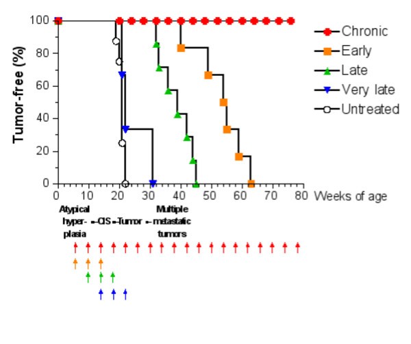
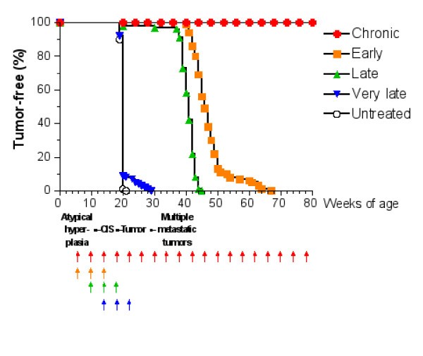
Tumor-free survival curves of HER-2/neu transgenic mice receiving the Triplex vaccine according to different protocols from [6]. Each arrow at the bottom of the graph represents one cycle of vaccination. The sequence of neoplastic progression in untreated mice is outlined under the x axis; CIS, carcinoma in situ.
The question whether the Chronic protocol is the minimal vaccination protocol yielding complete protection from tumor onset, or whether a lower number of vaccination cycles would provide a similar degree of protection is still an open question. Finding an answer to this question via a biological solution would be too expensive in time and money as it would require an enormous number of experiments, each lasting at least one year. For this reason we developed an accurate model of immune system responses to vaccination and we use this model as a virtual laboratory to search for effective vaccination protocols. The paper is organized as follows: section §2 will introduce the general requirements needed to model the problem; section §3 describes in details our virtual laboratory, i.e. the model, its structure and biological details, and its computer implementation (the simulator). In section §4 we present in silico experiments for different vaccination schedules and we show how the virtual laboratory can be used for designing a new and better protocol. Finally in section §5 we discuss our results, draw some conclusions, and plans for future investigations.
2 The general framework for modelling
In dealing with modelling of cancer – immune system interaction and competition one should be aware that this competition can play a crucial role besides therapeutical actions. This competition may possibly end up either with the elimination of the cancer cells, or the progressive invasion by cancer cells of other tissues or organs.
The goal of medical treatments is to enhance the immune response by activating the immune defense and/or specializing the ability of immune cells to identify the presence of the tumor.
The immune competition is a phenomenon which involves aggressive cells or particles (either external non-self pathogens or self modified or corrupted cells) and the various populations of the immune system. The immune system appears to be a distributed system which lacks central control, but which, nevertheless, performs its complex task in an extremely effective and effcient way. Complexity, in this framework, is driven by the fact that interactions are developed at different scales (i.e. the cellular dynamics is ruled by sub-cellular interactions) and different mechanisms operate on the same subject (mechanical for the dynamics and biological for the immune competition). The state of the art of the immune mechanisms from the view point of molecular biology are described in specialized literature [9, 10, 11]. Owing to the rapid progress of biological knowledge this is rapidly changing.
A model, which is a mapping from a real-world domain to a mathematical domain, highlights some of the essential properties while ignoring not relevant (or believed not relevant) ones. A good model must be relevant, capturing the essential properties of the phenomenon, computable, driving computational knowledge into mathematical representation; understandable, offering a conceptual framework for thinking about the scientific domain; and extensible, allowing the discovery of additional real properties in the same mathematical framework.
In the framework of immune system competition, relevant means that a model should be able to capture the essential properties of the system, the system entities organization and their dynamic behavior. A computable model should then be able to simulate both the dynamic behavior and the evolution and interactions of the system entities which play the game. An understandable model must reproduce concept and ideas of tumor immunology while opening new computational possibilities for understanding the immune competition. Finally extensible models should allow the inclusion of new knowledge with a limited effort. The immune system is characterized by a great complexity so that it is very diffcult, or even impossible, to develop a detailed mathematical description of all phenomena related to the immune competition which satisfies all the above properties. A significant effort has recently been devoted in searching for an appropriate mathematical approach to describe the Immune System – tumor competition (see [12] for a recent review). However, if one focuses the attention on specific types of interactions, one may attempt to develop ad hoc models for a specific phenomenon at the chosen observation and representation scale. Extensive description of subcellular vs larger scales of modelling can be found in [13, 14, 15]. Methods based on generalized kinetic model look very promising for system description: however they are not yet so detailed to model a specific therapeutic vaccine.
3 SimTriplex Model
To model the action of a specific tumor vaccine, we used a computational approach which reproduces the ab initio kinetic model that describes the interactions and diffusion of each relevant biological entity. This approach is biologically very flexible; the behavior of entities is modelled using present biological knowledge and can be easily modified to reflect observations from new biological experimental results. Compared to the complexity of the real biological system our model is still very naive and it can be extended in many aspects. However the model is complete enough to describe the major aspect of the phenomenon and, after tuning the model parameters, it can predict the response to a vaccination schedule that prevented the formation of solid tumors in mice.
Our model, hereafter referred as SimTriplex model, describes the immune competition using an agent based method. These methods are nowadays very popular as they find application in various fields. However the idea of discrete agents whose global dynamics is able to reproduce macroscopic behavior has been introduced more than fifty years ago in the framework of fluid-dynamics.
We used a Lattice Gas Automata (LGA) approach which allows to describe, in a defined space, the immune system entities with their different biological states and the interactions between different entities. The immune system evolution in a 2D physical space and in time is generated from the interactions and diffusion of the different entities. Extension to a 3D physical space is possible, but it would obviously have an higher computational cost. The major advantage of this technique is that the entities and the relationships can be described in terms that are much similar to the biological world. The intrinsic non linearity of the system is treated with no additional efforts. Models based on this class of techniques reproduce the biological knowledge of the system; so they are relevant, understandable and extensible. They are naturally computable but the computational effort increases drastically with increasing biological details (e.g. the immune repertoire and biological details). This class of model can be seen as the computational counterpart of the generalized kinetic model.
To describe the cancer – immune system competition one needs to include all the entities (cells, molecules, adjuvants, etc.) which biologists recognize as relevant in the competition. These entities have internal states, birth, age and death (i.e. ages structure). Interactions between different entities will stochastically change the internal state of one or both the interacting entities. Space changes in the system are achieved with diffusion instead of collision (see 3.2.4). It is worth to remind that in the microscopic cellular framework one is interested only in the initial and final state. The model of the mechanisms which produce the change of state is deferred to sub-cellular models.
Our model is driven by the experimental data on Triplex, an engineered vaccine for mammary carcinoma tested on HER-2/neu transgenic mice.
List of symbols and half life. Half life is expressed in times teps; one times tep represents 8 hours.
entity |
symbol |
half life |
|---|---|---|
B Cells |
B |
3.33 days |
Antibody Secreting Plasma Cells |
PLB |
10 |
T-helper lymphocytes |
TH |
10 |
T-cytotoxic lymphocytes |
TC |
10 |
Macrophages |
MP |
3.33 days |
Dendritic Cells |
DC |
10 |
Interleukin-2 |
IL-2 |
5 |
Immunoglobulins |
IgG |
5 |
Danger Signal |
D |
5 |
Major Histocompatibility Complex Class I |
MHCI |
- |
Major Histocompatibility Complex Class II |
MHCII |
- |
Tumor Associated Antigens |
Ag |
3 |
Immunocomplexes |
IC |
100 |
Cancer Cells |
CC |
1095 |
Vaccine Cells |
VC |
5 |
Natural Killer Cells |
NK |
10 |
Interleukin-12 |
IL-12 |
5 |
3.1 Entities Representation
The primary function of the immune system is a recognition function. Working at cellular scale we need to represent only those characteristics of entities which are relevant for recognition and interaction: state, recognition site and lifetime.
From the computational point of view, the major difference between cellular and molecular entities is that cells have a state attribute and may be classified on the basis of these attributes. Entities with no biological state, like antibodies are not followed individually, instead we consider only their total number for each lattice point. Their age structure is obtained increasing or decreasing the population number. Antigens (Ag or TAA) are however followed as individuals for their specific role.
Entities with biological states, i.e. cellular entities, are tracked individually in order to keep track of state change owing to interactions. The state of a cell is an artificial label introduced by the logical representation of the cells behavior. They have a standard lifetime which can eventually increase with interactions.
Most cellular and molecular entities have recognition sites (receptors). The set of lymphocyte's receptors is represented by bit-strings of length h [17] which then forms the so called "shape space" [18]. A clonal set of cells is characterized by the same clonotypic receptor, i.e. by the same bit-string of length l. The potential repertoire of receptors scales as 2 l .
Simple entities, like antibodies, are represented using their binding site (receptors). Tumor associated antigens are also described using their binding site but we keep also track of their lifetime. Representation of cellular entities include receptors, binding site and lifetime.
The receptor-coreceptor binding among the entities are described in terms of matching between binary strings with fixed directional reading frame. Bit-strings represent the generic "binding site" between cells (through their receptors) and target molecules (through peptides and epitopes). Every cellular entity is represented by a number of molecules, including the receptor. The repertoire is then defined as the cardinality of the set of possible instances of entities that differ in, at least, one bit of the whole set of binary strings used to represent its attributes.
Indeed, the cells equipped with binding sites and the antibodies, have a potential repertoire of
 , where N
e
indicates the number of binary strings used to represent receptors, MHC-peptide complexes, and epitopes of the entity e. Other entities do not need to be specified by binary strings so their repertoire is represented by a single entity (i.e. N
e
= 0). Examples include cytokine molecules such as interferon-γ and the danger signal [19].
, where N
e
indicates the number of binary strings used to represent receptors, MHC-peptide complexes, and epitopes of the entity e. Other entities do not need to be specified by binary strings so their repertoire is represented by a single entity (i.e. N
e
= 0). Examples include cytokine molecules such as interferon-γ and the danger signal [19].
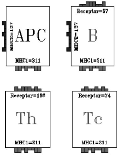
Grafical representation of lymphocytes and antigen presenting cells.
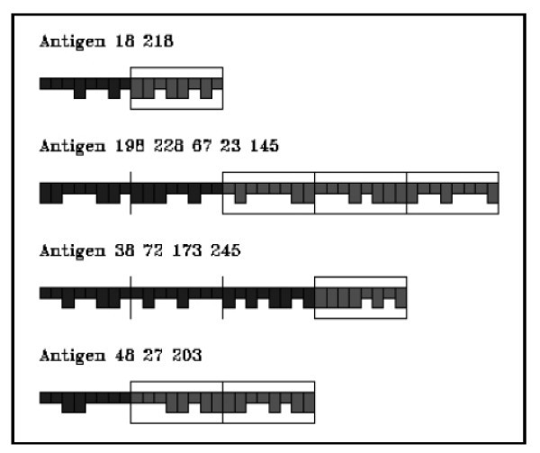
Graphical representation of antigens.
As receptors' entities are represented by bit strings, the only information available is a "similarity" between bit strings. A standard measure of similarity between two bit strings is the so called Hamming distance which is just the number of mismatching bits 2. The interactions between two entities equipped with receptors are defined by a probability measure, called affnity potential, which is a function of the Hamming distance between the binary strings representing the two entities' binding site. For two strings s and s' such probability is max when all corresponding bits are complementary (0 ↔ 1), that is, when the Hamming distance between s and s' is equal to the bit string length. If l is the bit string length and m is the Hamming distance between the two strings, the affnity potential is defined in the range 0, . . ., l as
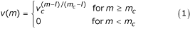
where v c ∊ (0,1) is a free parameter which determines the slope of the function where as m c (l/2 <m c ≤ l) is a cut-off (or threshold) value below which no binding is allowed.
The cells are free to diffuse across the lattice sites. At each time-step, representing 8 hours of real time, the cells and molecules residing on the same lattice site they can interact each other. The tissue is represented as two-dimensional triangular lattice (six neighbor sites) L × L, with periodic boundary conditions in both directions (up-down, left-right). The lattice is taken to represent here a portion of mammary tissue of the mouse.
All various classes of immune functional activity, phagocytosis, immune activation, opsonization, infection and cytotoxicity are described by computational rules.
The model also includes the mechanism of haematopoiesis as described in [16]. The rules which implement these actions are executed in a randomized order.
3.2 Coding SimTriplex
The high-level architecture of the code can be explained using the following pseudo-code.
SimTriplex Simulator
Input: Accept pre-determined inputs (e.g., user-specified vaccine injections, random generation of new B- and T-cells, etc.).
Time cycle start
Activate Thymus and Bone Marrow functions.
Haematopoiesis function is activated and operates for all cycles.
Interaction-driven dynamics. Enables the pairing of entities and modification of their states, creates new entities in response to these interactions, etc. in response to these interactions.
Internal dynamics. Makes allowance for internal, non interaction-driven dynamics (e.g. aging and natural death, differentiation, mutation, etc.).
Diffusion. Allows cellular entities to diffuse on the lattice checking the physical space constraints. Change the density of molecular entities in order to mimic diffusion.
Output. Stores a trace of the state of the system at time t.
Time cycle ends
code end
A set-up routine will create the lattice, register the values of the various input parameters and stochastically fill the lattice with all population of cells. Time step interactions will proceeds up to a preselected final time.
Cellular and molecular entities are treated differently in the model. Cellular entities are treated individually while molecular entities are modelled as populations. We describe them separately.
3.2.1 Cellular entities
The common features of cellular entities are : Position, Specificity, States and Age.
Position is the crucial parameter which defines which entities can interact as interactions between entities can occur only between those entities which are co-located in the same lattice cell;
In the shape space [17] entities interact according to their specificity represented by binary string. This simulates recognition of the entities by their paratopes (complementary shapes of peptides and receptors). Each entity, except for plasma cells, has at least one receptor (or paratope/epitope, depending on whether they are cellular or molecular entities) which is its primary identifier, i.e., its specificity.
The key constituents of specificity are MHC class I (MHC-I) and MHC class II (MHC-II), T cell receptors (TCR) and B-cell receptors (BCR). The different class of cellular entities we consider are: B-cells, T helper cells (TH), cytotoxic T cells (TC), antigen presenting cells (APC) and plasma cells (PLB). B cells are endowed with MHC-II and BCR; TC cells are equipped only with TCR (CD8) and TH include TCR (CD4).
With the name APC cells one refers to Macrophages (MP), Dendritic cells (DC) and B-cells. MP are aspecific APC and do not contain any specific receptor. They phagocytose antigens (in our case TAA) and expose their bit string as MHC-II. DC are also aspecific APC. They internalize TAA and expose as MHC-I and MHC-II. Finally B-cells act as specific APC. If they recognize TAA they internalize it and expose as MHC-II. Plasma cells have no specific receptor (but contains the information of the original BCR). They produce antibodies with the same receptor as the B cell from which they originate.
Entities' states. Internal states (columns) of each cell type (rows) are labelled with a •. The rows show the states of each entity.
Cell |
Active |
Re-sting |
Intern |
PresI |
PresII |
Duplica |
Bound-ToAb |
|---|---|---|---|---|---|---|---|
B |
• |
• |
• |
• |
• |
||
TH |
• |
• |
• |
||||
TC |
• |
• |
• |
||||
DC |
• |
• |
• |
• |
• |
||
MP |
• |
• |
• |
• |
|||
CC |
• |
• |
• |
||||
VC |
• |
• |
|||||
NK |
• |
Each cells can be in different internal states and all cells are tracked individually throughout the course of an experimental run. In order to describe state changes we will look (see § 3.2.3) at the evolutions of each cellular entity since its initially entry in the lattice. Here we briefly describe the biological meaning of entities states.
APC, TH and B cells are initialized as Active; TC cells are initialized as Resting; VC are initialized as PresI while CC are stochastically set as PresI with an high probability. All entities are initialized with their default life time (see Age).
All cellular entities will then change their status following a successful interaction with another entity (hereafter referred as positive interaction) or by internal processing. Conditions under which a positive interaction (or the opposite negative interaction) occurs will be described later (see § 3.2.3).
-
APC (MP, DC and B cells) will change their status to Intern when they interact positively with TAA; Internal processes will then change the state to PresI (MHC class I) or PresII (MHC class II). DC may present both in MHC-I and MHC-II. Positive interaction of a presenting MHC-II APC with an active TH cell will change both B cells APC and TH state to Duplica and clonal proliferation phase begins for B cells. If a PresII APC negatively interacts with a TH cell, its status can return to Active. This simulates the biological event that a presenting APC that is not stimulated by TH-cell may loose the presentation status.
-
B cells change their status only when they positively interact with a TAA or with a TH cell as described above.
-
Cytotoxic T cells become Active when positively interact with a presenting MHC-I DC, or with a VC in presence of IL-12 adjuvant or with a CC in presence of IL-2 previously released by an activated TH cell. Active TC cells can recognize and kill a CC by lysis. In such a case, the status of the TC changes to Duplica and clonal division starts.
-
Helper T cells change their status only when they positively encounter an APC as described above.
-
Cancer and vaccine cells positively interact with Antibodies and change their status to BoundToAb.
Antibodies can then kill them by complement mediated cytotoxicity or can act as signals for NK cells. Cellular entities have age structure. They are born, they interact and duplicate (and eventually get anergic) and, after a finite lifetime, they die by apoptosis or by lysis. We need to keep track of the age of cellular entities; we do this by keeping a count of the number of time-steps since cell birth (from stem cells or by clonal division). To simulate memory cells, we increase the halflife of TH, TC and B cells after successful interaction with target antigens. The death probability reaches 1 when the age gets to twice the half life. The simulator performs the process of the thymic selection of T cells (TH + TC) as described in [16]. Selection has two phases: negative and positive (both stochastic).
The simulated immune system achieves repertoire completeness by a mechanism of mutation of B-cell receptor (BCR). Mutation occurs when a new B cell is formed, i.e. in the duplication phase. This effect is included in the simulator as a stochastic event; this increases the immune system recognition ability. The setup routine initially set entities concentration in the lattice. The Leukocytes form three general classes (Granulocytes; Lymphocytes and Monocytes) which are present in different ratios in blood, tissues and various organs. In our virtual mouse we initially consider 4500 leukocytes. Of these there are 4200 lymphocytes, comprising 1512 B cells, 1512 T cells (subdivided in 1008 T helper cells and 504 cytotoxic T cells) and 1176 natural killer cells. There are 300 monocytes divided in 150 macrophages and 150 dendritic cells. The model does not have any granulocyte.
3.2.2 Molecular entities
Molecular entities included in the simulator are Antigens, Antibodies, Cytokines and Damage (Danger Signal, see [19]). Molecular entities do not have internal states and thus do not need to be modelled individually (only TAA are treated individually). Rather, we define populations which represent different specificity of molecular entities, on the lattice. Diffusion on the lattice is performed by appropriate change of the concentrations of entities on the lattice. The age structure is stochastically increased/decreased as function of production and half life time respectively.
As antigen we consider only the tumor associated antigen (p185) released by injected vaccine cells and cancer cells when they die. Antigens are represented by a number of binary segments consisting of a fixed number of bits. These segments represent the antigenic sites (epitopes and peptides) as shown in Figure 3. Epitopes are defined as the external portion of an antigen that is recognized by a B-cell receptor. Peptides are defined as portions of an antigen that can be bound by an MHC molecule and be recognized by an appropriate T cell. The epitopes and peptides are specified separately in the model. The minimum effective antigen we consider is therefore two segments long, one for B-cell epitope and one for peptide.
Antibodies (Ab) are also represented by bit strings, and have a paratope which is identical to the paratope/receptor of the B cell (plasma cell) that secretes them.
Cytokines (IL-2 and IL-12) and a danger signal are encoded as aspecific entities. Their presence in the lattice site will induce or prevent interactions by increasing or decreasing probabilities.
3.2.3 Interactions
In this section we will describe interactions following the evolution of the simulator for the first few steps. First of all we must remember that interactions occurs only if two entities stay in the same site. Taking into account that a time step is 8 hours we can say that entities in a site are those entities that a single entity encounters during 8 hours. Time t = 0 corresponds to the atypical hyperplasia, i.e. first appearing of tumor cells. For "early schedule" time t = 0 corresponds also to the first vaccine injection. An interaction between two entities is a complex action which eventually end with a state change of one or both entities. Interactions can be specific or aspecific. Specific interactions need a recognition phase between the two entities (e.g. B ↓ TAA); recognition is based on Hamming distance and affnity function and is eventually enhanced by adjuvants. We refers to positive interaction when this first phase occurs successfully. Aspecific interaction do not have a recognition phase (e.g. DC ↓ TAA). When two entities, which may interact, lie in the same lattice site then they interact with a probabilistic law. All entities which may interact and are in the same site have a positive interaction.
Simulator's interactions. An interaction between two entities occurs if the row/column interaction is marked with a •. The table is obviously symmetric.
|
Entity 1 Entity 2 |
B |
Ag |
Ab |
TH |
TC |
MP |
DC |
IC |
VC |
CC |
NK |
|---|---|---|---|---|---|---|---|---|---|---|---|
B |
• |
• |
|||||||||
Ag |
• |
• |
• |
• |
|||||||
Ab |
• |
• |
• |
• |
|||||||
TH |
• |
• |
• |
||||||||
TC |
• |
• |
|||||||||
MP |
• |
• |
• |
||||||||
DC |
• |
• |
|||||||||
IC |
• |
||||||||||
VC |
• |
• |
• |
||||||||
CC |
• |
• |
• |
||||||||
NK |
• |
• |
• |
• |
3.2.4 Diffusion
All entities are allowed to move with uniform probability between neighboring lattices in the grid with equal diffusion coeffcient. In the present release of the simulator chemotaxis is not implemented.
4 Results
The systematic search for a new schedule is driven by the known in vivo results that we have reproduced with our model. In the following we first describe how we set up our virtual lab in-silico experiments which reproduced the in vivo results (section § 4.1); we then analyze results of the different schedules with to analyze the immune system reaction to vaccine injections (section § 4.2). Finally, by taking into account what we learned from computer experiments, we systematically search for a new schedule alternative to the chronic one, which could prevent the solid tumor formation (section 4.3).
4.1 Setting in silico experiments
In vivo experiments on sets of HER/2-neu mice have been carried, for all the schedules, up to the time in which a solid tumor is formed in the mouse. In fact, one observes that the effectiveness of vaccine action is depleted after a solid tumor is formed. In order to mimic these experiments in silico one needs to define a solid tumor on a lattice. Taking into account the number of simulated Immune System entities in the lattice we assume that a solid tumor is formed when the number of cancer cells in the lattice becomes greater than 105.
The vaccination protocols that have been used to test the effectiveness of Triplex are described in section 1. In in silico experiments we try to reproduce in vivo experiments. For this we considered all the different protocols mentioned above and the case of untreated mice. The last one is analyzed in order to tune with experimental tumor growth and ensure that simulation shows no significant immune response.
We performed in silico experiments using the standard good practice statistical procedure: i) We considered a large population of individual mice. Each individual mouse is characterized by a sequence of uniform numbers which will determine the probabilistic events. ii) We randomly extract from this population two statistical samples of 100 individual mice (hereafter referred as S 1 and S 2) to perform numerical experiments.
Tumor-free survival curves of virtual mice receiving the Triplex vaccine according to different protocols. Each arrow at the bottom of the graph represents one cycle of vaccination. The sequence of neoplastic progression in untreated mice is outlined under the x axis; CIS, carcinoma in situ.
4.2 Analysis of schedules' results
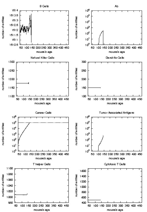
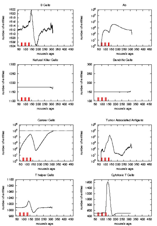
Immune response. The immune response activation is shown for untreated virtual mice, versus time in days.
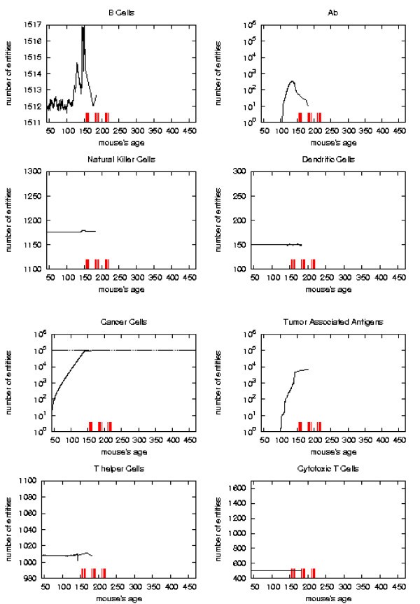
Immune response. The immune response activation due to the vaccine effect is shown for VERY LATE vaccination schedules, versus time in days. Red ticks above x axis represent the timing of vaccine administration.
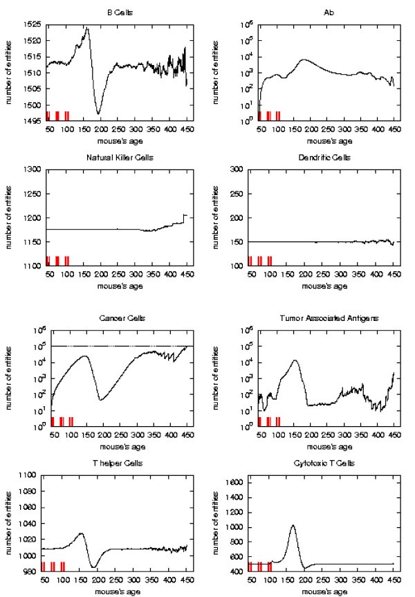
Immune response. The immune response activation due to the vaccine effect is shown for EARLY vaccination schedules, versus time in days. Red ticks above x axis represent the timing of vaccine administration.
Immune response. The immune response activation due to the vaccine effect is shown for LATE vaccination schedules, versus time in days. Red ticks above x axis represent the timing of vaccine administration.
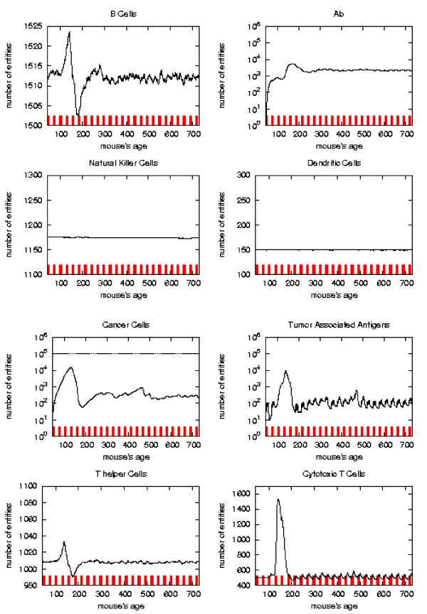
Immune response. The immune response activation due to the vaccine effect is shown for CHRONIC vaccination schedules, versus time in days. Red ticks above x axis represent the timing of vaccine administration.
The error analysis shows that in the regions where the sample has strong statistical significance (i.e. there still is a suffcient large number of mice which has not formed a solid tumor), the standard deviation always reaches a maximum of 5–8% for all entities.
First of all we notice that very late and untreated protocols show similar curves. Thus very late schedule is not relevant as it does not affect tumor growth. We will not discuss further this schedule.
Early and late protocol show a similar general behavior for all quantities. The chronic protocol shows a behavior which is different from all the others protocols.
This last three schedules show an initial transient phase characterized by a strong cytotoxic response which corresponds to a drastic reduction of cancer cells. This initial, burst like, transient phase appears also, for all the three schedules, in T helpers, cytotoxic T cells, B cells and antibodies. The antibodies grow immediately after the first vaccine injection. This effect is due to the antibodies released by vaccine cells. The general behavior is similar for all the schedules but there are significant differences:
i) the vaccine's effect on the growth of cancer cells appears after the second cycle of vaccination;
ii) cancer cells drop off roughly two months after the end of the early schedule, while in the late protocol the drop begins in between second and third cycle of vaccination;
iii) the same delay can be observed in the other entities behavior (except for natural killer and dendritic cells as explained in [16]);
iv) Cytotoxic T cells response is higher in late protocol than in early one. This is probably due to the fact that in late vaccination there are many more cancer cells than in the early;
v) Antibody response is more powerful in early than late. This is crucial for controlling tumor progression [6]: early treated mice survive about 20 weeks more than late treated mice. Early protocol is then successful in delaying the formation of the solid tumor via humoral response.
As already mentioned chronic schedule plots show a transient phase as in other schedules. This is followed by a quasi steady phase. All the plots, during the quasi steady phase, are mostly flat and characterized by small humps with maximum at the end of each vaccination cycle. The number of antibodies, after the initial increase, keeps constant. This show, as found in the in vivo data, that cancer growth is controlled by antibodies. The number of cancer cells is always in the range 103 ÷ 104.
4.3 Computer aided search for a new schedule
The search for a new schedule can be envisaged from the results, previously shown, of the three protocols giving, at least, an initial positive response, i.e. early, late and chronic.
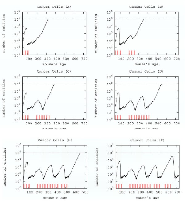
Searching a new schedule: results after early cycles for a single mice. Red ticks above x axis represent the timing of vaccine administration.
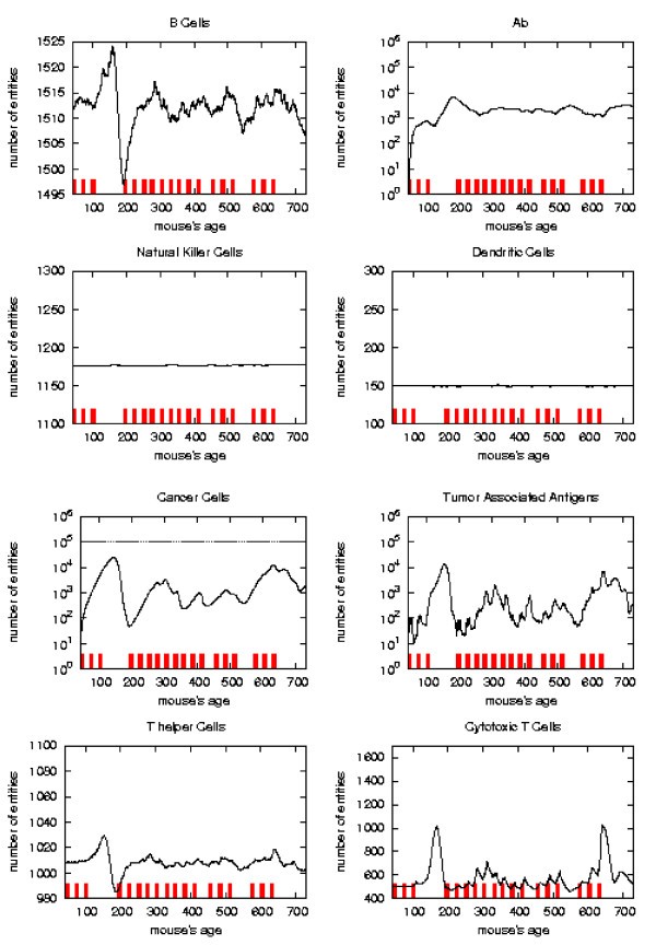
Immune response. The immune response activation due to the vaccine effect is shown for a possible vaccination schedules, versus time in days. Red ticks above x axis represent the timing of vaccine administration.
This schedule is able to control the tumor formation with a number of vaccine injections 30% less than the chronic one.
5 Conclusion
We presented an in silico search for effective cancer vaccination protocols using a model describing the action of a tumor vaccine in stimulating immune response and the ensuing competition between the immune system and tumor cells. This model applies to the very early stage of tumor genesis, i.e. before a solid tumor is formed. In silico experiments show excellent agreement with in vivo experiments both for the time of formation of solid tumor in mice and the role of antibody response in controlling tumor growth [6, 8]. The model and its computer implementation are very flexible and new biological entities, behavior, and interactions can be easily added. This helps achieving a realistic description of the immune responses that target solid tumor formation.
We found that a possible protocol which prevents solid tumor formation for the mice lifetime and uses a number of vaccine injections 30% less than Chronic schedule. This result shows that, at least in principle, a computerized mathematical model can be used to search for better protocols. The vaccination schedule we found is better than the Chronic one. However the question if this schedule is optimal, i.e. is the effective schedule with the minimum number of injections, or nearly-optimal is still open. The answer to this question is not trivial. First one should properly define the biological meaning of an optimal schedule; then an optimal/nearly optimal solution can be found with different techniques available in the mathematical market. We plan to further investigate this point using alternative strategies, or optimal search algorithms like simulated annealing or genetic algorithms, taking into account biological constraints.
Moreover the model we used is still naive and can be improved greatly. We are working to a more detailed model to dissert the contribution of individual vaccine's components to the protective immune response. We plan also to consider a multi-organ model in order to consider metastasis formation, and the vaccine's effect on metastasis. Work in these directions is in progress and results will be published in due course.
Declarations
Acknowledgements
F.P. and S.M. acknowledge partial support from University of Catania research grant and MIUR (PRIN 2004: Problemi matematici delle teorie cinetiche). Part of this work has been done while F.P. is research fellow of the Faculty of Pharmacy of University of Catania.
P.-L.L. acknowledges financial support from the University of Bologna, the Department of Experimental Pathology ("Pallotti" fund) and MIUR.
Authors’ Affiliations
References
- Rosemberg SA, Yang JC, Restifo NP: Cancer immunotherapy: moving beyond current vaccines. Nat Med 2004,10(9):909–915.View ArticleGoogle Scholar
- Forni G, Lollini PL, Musiani P, Colombo MP: Immunoprevention of cancer: is the time ripe? Cancer Res 2000,60(10):2571–2575.PubMedGoogle Scholar
- Chang MH, Chen CJ, Lai MS, Hsu HM, Wu TC, Kong MS, Liang DC, Shau WY, Chen DS: Universal hepatitis B vaccination in Taiwan and the incidence of hepatocellular carcinoma in children. N Engl J Med 1997,336(26):1855–1859.View ArticlePubMedGoogle Scholar
- Koutsky LA, Ault KA, Wheeler CM, R BD, Barr E, Alvarez FB, Chiacchierini LM, Jansen KU: Proof of Principle Study Investigators. A controlled trial of a human papillomavirus type 16 vaccine. N Engl J Med 2002,347(21):1645–1651.View ArticlePubMedGoogle Scholar
- Di Carlo E, Diodoro MG, Boggio K, Modesti A, Modesti M, Nanni P, Forni G, Musiani P: Analysis of mammary carcinoma onset and progression in HER-2/neu oncogene transgenic mice reveals a lobular origin. Lab Invest 1999,79(10):1261–1269.PubMedGoogle Scholar
- Lollini PL, De Giovanni C, Pannellini T, Cavallo F, Forni G, Nanni P: Cancer immunoprevention. Future Oncology 2005, 1:57–66.View ArticlePubMedGoogle Scholar
- Colombo MP, Trinchieri G: Interleukin-12 in anti-tumor immunity and immunotherapy. Cytokine Growth Factor Rev 2002,13(2):155–168.View ArticlePubMedGoogle Scholar
- De Giovanni C, Nicoletti G, Landuzzi L, Astolfi A, Croci S, Comes A, Ferrini S, Meazza R, Iezzi M, Di Carlo E, Musiani P, Cavallo F, Nanni P, Lollini P: Immunoprevention of HER-2/neu transgenic mammary carcinoma through an interleukin 12-engineered allogeneic cell vaccin. Cancer Res 2004,64(11):4001–4009.View ArticlePubMedGoogle Scholar
- Delves PJ, Roitt YM: The immune system. Advances in Immunology 2000, 343:37–49.Google Scholar
- Forni G, Foa R, Santoni A, Frati L, Eds: Cytokine Induced Tumor Immunogeneticity New York: Academic Press 1994.Google Scholar
- Greller L, Tobin F, Poste G: Tumor hetereogenity and progression: conceptual foundation for modeling. Invasion and Metastasis 1996, 16:177–208.Google Scholar
- Bellomo N, De Angelis E, Preziosi L: Multiscale Modeling and Mathematical Problems Related to Tumor Evolution and Medical Therapy. Journal of Theoretical Medicine 2003,5(2):111–136.View ArticleGoogle Scholar
- Bellomo N, Preziosi L: Modelling Mathematical Methods and Scientific Computation Boca, Raton: CRC Press 1995.Google Scholar
- Bellomo N, Pulvirenti M: Modeling in Applied Sciences: A Kinetic Theory Approach Birkhauser, Boston 2000.Google Scholar
- Motta S, Brusic V: Modelling in Molecular Biology Springer 2004 chap. Mathematical modelling of the immune system 193–218.Google Scholar
- Pappalardo F, Lollini PL, Castiglione F, Motta S: Modelling and Simulation of Cancer Immunoprevention vaccine. Bioinformatics 2005,21(12):2891–2897.View ArticlePubMedGoogle Scholar
- Farmer JD, Packard N, Perelson AS: The immune system, adaption and machine learning. Phisica D 1986, 22:187–204.View ArticleGoogle Scholar
- Segel LA, Perelson AS: Some reflections on memory in shape spaces Springer Coll of Theories of Immune Networks 1989, 63–70.Google Scholar
- Matzinger P: An innate sense of danger. Immunology 1998, 10:399–415.Google Scholar
Copyright
This article is published under license to BioMed Central Ltd. This is an Open Access article distributed under the terms of the Creative Commons Attribution License (http://creativecommons.org/licenses/by/2.0), which permits unrestricted use, distribution, and reproduction in any medium, provided the original work is properly cited.